66
and Ramankutty 1994 ). Here, data from HadSST3.1.1.0 have been used (same cita-
tions and web address as for ENSO). As shown in the Supplement of Canty et al.
( 2013 ), nearly identical scientific results are obtained using SST from NOAA. The
AMV index is a proxy for changes in the strength of the Atlantic Meridional
Overturning Circulation (AMOC) (Knight et al. 2005 ; Stouffer et al. 2006 ; Zhang
et al. 2007 ; Medhaug and Furevik 2011 ). Others use Atlantic Multidecadal Oscillation
(AMO) to describe this index, but we prefer AMV because whether or not the strength
of the AMOC varies in a purely oscillatory manner (Vincze and Jánosi 2011 ) is of no
consequence to the use of this proxy in the EM-GC framework.
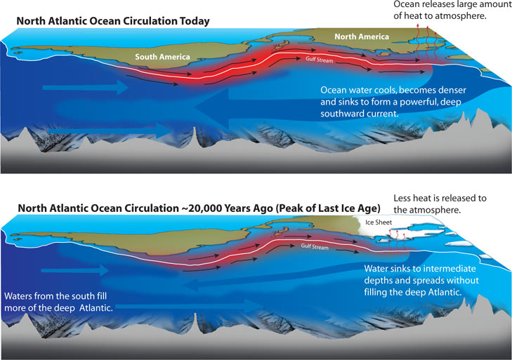
There are two important details regarding AMVi that bear mentioning. This index
represents the fact that, during times of increased strength of the AMOC, the ocean
releases more heat to the atmosphere.^12 There is considerable debate regarding
whether the strength of AMOC varies over time (e.g., Box 5.1 of IPCC ( 2007 ) and
Willis ( 2010 )). Our focus is on anomalies of AMOC over time; hence, the AMVi
index is de-trended.^13 As shown in Fig. 5 of Canty et al. ( 2013 ), various choices for
how this index is de-trended have considerable effect on the shape of the resulting
time series, which is important for the EM-GC approach. Here, total anthropogenic
ΔRF of climate is used to de-trend AMVi, because this method appears to provide a
more realistic means to infer variations in the strength of AMOC from the North
Atlantic SST record than other de-trending options (Canty et al. 2013 ). The second
detail involves whether monthly data should be used for the AMVi index, since the
AMOC is sluggish and variations of North Atlantic SST on time scales of a year or
less likely do not represent variations in large-scale, ocean circulation. Throughout
this chapter, the AMVi index has been filtered to remove all components with tempo-
ral variations shorter than 9 years; only variations of SST on time scales of a decade
or longer are preserved. The interested reader is invited to examine Fig. 7 of (Canty
et al. 2013 ) to see the impact of various options for how AMVi is filtered.
A major international research effort has provided new insight into temporal
variations of the strength of AMOC (Srokosz and Bryden 2015 ). The RAPID-
AMOC program, led by the Natural Environment Research Council of the United
Kingdom, is designed to monitor the strength of the AMOC by deployment of an
array of instruments at 26.5°N latitude, across the Atlantic Ocean, which measure
temperature, salinity and ocean water velocities from the surface to ocean floor
(Duchez et al. 2014 ). Analysis of a 10 year (2004–2014) time series of data reveals
a decline in the strength of AMOC over this decade, similar to that shown by our
proxy (AMOC ladder, Fig. 2.5) over this same period of time.
(^12) An illustration of the physics of the interplay between AMOC and release of heat to the atmo-
sphere from the ocean is at http://www.whoi.edu/cms/images/oceanus/2006/11/nao-en_33957.jpg
(^13) The de-trending of AMV, the proxy for variations in the strength of AMOC, means that when
examined over the entire 156 year record of the simulation, the slope of the panel marked AMOC
in Fig 2.5 is near zero. The proxy used to represent AMOC is based on measurements of sea sur-
face temperature, which rise over time due to the transfer of heat from the atmosphere to the ocean.
Within an MLR model such as the EM-GC, the AMOC proxy should be de-trended, or else a
number of erroneous conclusions regarding long-term climate change could result. See Sect. 3.2.3
of Canty et al. ( 2013 ) for further discussion.
2 Forecasting Global Warming